Education | Key Stats, Risk and Performance 101 Concepts

Hi All,

I wanted to cover some high-level basic concepts across key stats, risk, and performance measures. Will create a more in-depth concept pager for each later, but in the meantime, enjoy!

Key Concepts Covered:

• Normal Distribution
• Standard Deviation
• Key characteristics of normal distribution
• Regression Analysis
• Linear Regression
• P-value
• Vector
• R-squared
• Beta
• Correlation
• Covariance
• Value at Risk
• Can the standard deviation (volatility) be different from VaR of a portfolio?
• Analytical VaR
• Historical VaR
• Monte Carlo Simulation
• Shortfall Risk
• Bond Math
• Convexity
• Key Rate Duration (KRD)
• Bond Risk Measures
• Performance measures
• Other Suggested Resources

Normal Distribution

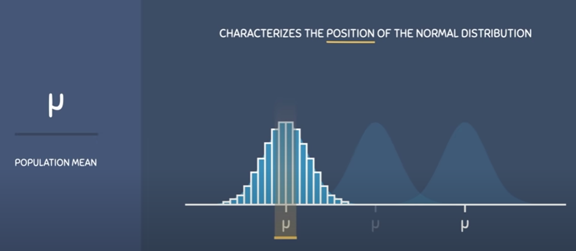
The normal distribution, also known as the Gaussian distribution, is a probability distribution that describes a continuous set of data that tends to cluster around a single mean or average value, with a symmetrical bell-shaped curve.

In a normal distribution, the mean, median, and mode are all equal and the distribution is characterized by two parameters: the mean (μ) and the standard deviation (σ). The shape of the normal distribution is determined by these parameters and the curve is symmetric around the mean.

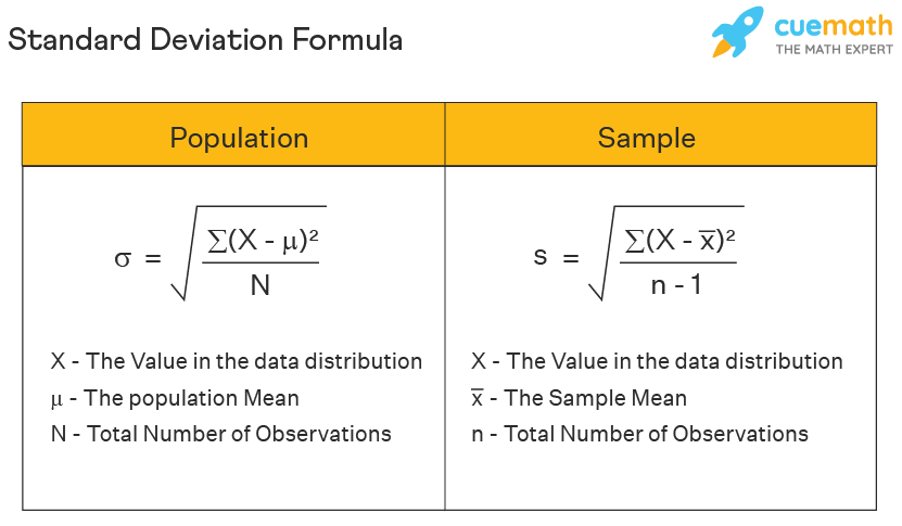
Note) It is important to make a distinction between sample vs. population.

Many real-world phenomena, such as height, weight, and IQ scores, follow a normal distribution. The normal distribution is also important in statistics because of the central limit theorem, which states that the sum of a large number of independent and identically distributed random variables will tend towards a normal distribution.

Standard Deviation

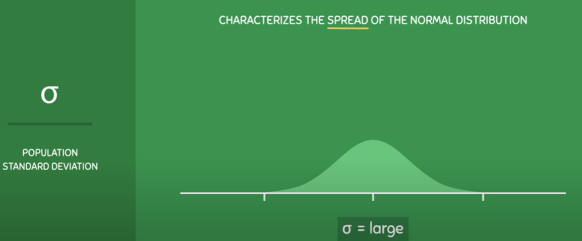
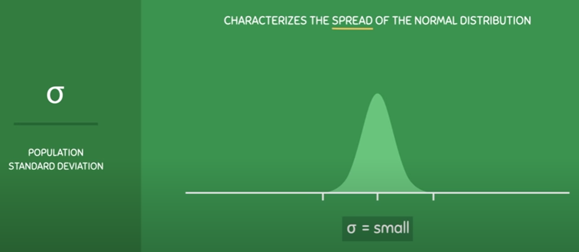
Standard deviation is a statistical measure of the amount of variation or dispersion in a set of data. It measures how much the values in a dataset vary (i.e. 'spread') from the mean or average value.

In other words, it tells you how spread out the data is. A small standard deviation indicates that the data is clustered around the mean, while a large standard deviation indicates that the data is more spread out.

The formula for calculating the standard deviation is the square root of the variance, which is the average of the squared differences from the mean. Standard deviation is often used in hypothesis testing, to determine the significance of differences between groups or to assess the variability within a group.

In practical terms, understanding the standard deviation of a dataset can help you to interpret and compare data, and to identify outliers or unusual data points.

Key characteristics of normal distribution

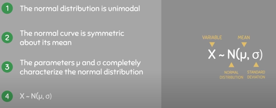
Source: The Normal Distribution and the 68-95-99.7 Rule (5.2)

Regression Analysis

Regression analysis is a statistical method used to examine the relationship between one or more independent variables and a dependent variable. The goal of regression analysis is to determine how changes in the independent variables are associated with changes in the dependent variable.

In a typical regression analysis, the researcher starts by collecting data on the independent variables and the dependent variable. The researcher then uses statistical software to fit a regression equation to the data, which can be used to estimate the effect of the independent variables on the dependent variable.

There are two main types of regression analysis: simple regression and multiple regression. Simple regression involves examining the relationship between a single independent variable and a dependent variable. Multiple regression involves examining the relationship between two or more independent variables and a dependent variable.

Regression analysis is commonly used in various fields such as economics, finance, psychology, and biology to study the relationships between variables and make predictions based on those relationships. It can also be used to identify outliers, test hypotheses, and estimate the magnitude and direction of the relationship between variables.

Use case in finance

Regression analysis is a useful tool for portfolio construction and investing, as it allows investors to better understand the relationships between different variables and to make more informed decisions about their investments.

For example, a portfolio manager may use regression analysis to estimate the expected return of a portfolio based on the historical returns of different asset classes (such as stocks, bonds, and real estate) and other relevant factors (such as interest rates, inflation, and economic growth). By analyzing the historical relationships between these variables, the portfolio manager can identify which factors have had the strongest influence on portfolio returns and use this information to make informed investment decisions.

Additionally, regression analysis can be used to evaluate the effectiveness of different investment strategies and to identify potential sources of risk or alpha. For instance, a portfolio manager may use regression analysis to test whether a particular factor, such as value or momentum, has a significant impact on the performance of a portfolio. If the analysis suggests that the factor does indeed have an impact, the portfolio manager may adjust the portfolio's asset allocation or investment strategy accordingly to take advantage of this insight.

Linear Regression

Linear regression analysis is a statistical method used to model the relationship between a dependent variable and one or more independent variables, with the assumption that this relationship is linear. In linear regression analysis, a straight line (or linear equation) is used to estimate the effect of the independent variables on the dependent variable.

The simplest form of linear regression analysis is simple linear regression, which involves examining the relationship between a single independent variable and a dependent variable. The linear equation used in simple linear regression takes the form of:

Y = a + bX

Where Y is the dependent variable, X is the independent variable, a is the intercept (the value of Y when X is zero), and b is the slope (the change in Y associated with a one-unit increase in X).

Multiple linear regression analysis involves examining the relationship between two or more independent variables and a dependent variable. The linear equation used in multiple linear regression takes the form of:

Y = a + b1X1 + b2X2 + ... + bnXn

Where Y is the dependent variable, X1, X2, ..., Xn are the independent variables, a is the intercept, and b1, b2, ..., bn are the slopes associated with each independent variable.

Linear regression analysis is commonly used in various fields to model relationships between variables, predict outcomes, and estimate the strength and direction of the relationship between variables. It can also be used to identify outliers and influential observations, test hypotheses, and evaluate the effectiveness of interventions.

P-value

In statistics, a p-value is a measure of the strength of evidence against a null hypothesis. The null hypothesis is a statement that there is no significant difference or relationship between two variables or populations.

The p-value is the probability of obtaining a result as extreme or more extreme than the observed result, assuming that the null hypothesis is true. A p-value is typically compared to a significance level, which is a predetermined threshold for rejecting the null hypothesis. If the p-value is less than or equal to the significance level, the null hypothesis is rejected in favor of the alternative hypothesis, which is a statement that there is a significant difference or relationship between two variables or populations.

For example, suppose a researcher wants to test whether there is a significant difference in mean scores between two groups. The null hypothesis is that there is no significant difference between the two groups, while the alternative hypothesis is that there is a significant difference. The researcher calculates a p-value of 0.03 and sets a significance level of 0.05. Since the p-value is less than the significance level, the null hypothesis is rejected in favor of the alternative hypothesis, and the researcher concludes that there is a significant difference in mean scores between the two groups.

The p-value is a useful tool for assessing the strength of evidence against a null hypothesis and can help researchers make decisions about whether to reject or retain the null hypothesis. However, it is important to note that a low p-value does not necessarily mean that the alternative hypothesis is true or that there is a strong effect. Other factors such as sample size and study design should also be taken into account when interpreting statistical results.

Use case in finance

p-values can be a useful tool for portfolio managers and investors to evaluate the significance of relationships between different variables and portfolio performance, and to make more informed investment decisions based on statistical evidence.

For example, a portfolio manager may use a regression analysis to test whether there is a significant relationship between interest rates and the performance of a bond portfolio.

• The null hypothesis, in this case, would be that there is no significant relationship between interest rates and portfolio performance,
• while the alternative hypothesis would be that there is a significant relationship.

After conducting the regression analysis, the portfolio manager may calculate a p-value of 0.03, which is lower than the commonly used significance level of 0.05. This means that there is strong evidence against the null hypothesis and that the relationship between interest rates and portfolio performance is statistically significant.

Based on this analysis, the portfolio manager may decide to adjust the portfolio's asset allocation or investment strategy to take advantage of this relationship. For example, if the analysis suggests that the portfolio performs better during periods of low-interest rates, the manager may increase the portfolio's exposure to lower-duration bonds or other interest rate-sensitive securities.

Vector

In regression analysis, a vector is simply a mathematical object that represents a set of numbers or values arranged in a specific order. In the context of regression analysis, vectors are often used to represent the independent and dependent variables in the regression equation.

For example, in a simple linear regression analysis with one independent variable, the regression equation would be of the form:

y = a + bx

where y is the dependent variable (e.g. portfolio returns), x is the independent variable (e.g. interest rates), a is the intercept (i.e. the value of y when x = 0), and b is the slope (i.e. the change in y for a unit change in x). In this equation, both y and x are represented as vectors of data points, which are typically arranged in columns in a data matrix.

In more complex regression analyses with multiple independent variables, vectors may be used to represent each of the independent variables and their associated coefficients. For example, in a multiple linear regression analysis with three independent variables (x1, x2, and x3), the regression equation would be of the form:

y = a + b1x1 + b2x2 + b3x3

In this equation, each of the independent variables (x1, x2, and x3) would be represented as a vector of data points, and each of the corresponding coefficients (b1, b2, and b3) would be represented as a vector of values that indicate the impact of each variable on the dependent variable (y).

Overall, vectors are a fundamental component of regression analysis, as they are used to represent the variables and coefficients that are used to model the relationship between different factors and portfolio performance.

R-squared

R-squared, also known as the coefficient of determination, is a statistical measure used in regression analysis to assess how well the regression equation fits the data. Specifically, R-squared measures the proportion of the variance in the dependent variable that can be explained by the independent variables in the regression equation.

The R-squared value ranges from 0 to 1, with higher values indicating a better fit of the regression equation to the data. A value of 0 indicates that the regression equation does not explain any of the variance in the dependent variable, while a value of 1 indicates that the regression equation explains all of the variance in the dependent variable.

For example, if the R-squared value in a linear regression analysis is 0.8, this means that 80% of the variance in the dependent variable can be explained by the independent variables in the regression equation. The remaining 20% of the variance is attributed to other factors that are not included in the regression equation.

In portfolio construction and investing, R-squared can be a useful tool for assessing the strength of the relationship between different variables and portfolio performance. A higher R-squared value indicates a stronger relationship, which may be more predictive of future portfolio performance. However, it is important to note that a high R-squared value does not necessarily imply causation, and that other factors not included in the regression equation may also affect portfolio performance.

Beta

In the context of portfolio construction and bond investing, beta is a measure of a bond's or a portfolio's sensitivity to changes in the broader market. Beta is a statistical measure that compares the volatility of a bond or a portfolio to the volatility of a benchmark, such as a market index like the S&P 500.

A bond or portfolio with a beta of 1 is said to have the same level of volatility as the benchmark. A beta of greater than 1 means that the bond or portfolio is more volatile than the benchmark, while a beta of less than 1 means that it is less volatile. For example, a bond with a beta of 0.8 is expected to be 20% less volatile than the benchmark.

Beta is a useful tool for investors because it helps them to understand the risk of a particular bond or portfolio relative to the broader market. Bonds or portfolios with higher betas are generally considered to be riskier, as they are more sensitive to market fluctuations, while bonds or portfolios with lower betas are considered to be less risky.

Investors can use beta to manage the risk of their bond portfolios by selecting bonds with betas that are consistent with their overall risk tolerance and investment objectives. For example, investors who are looking to minimize risk might choose bonds with low betas, while investors who are looking to maximize returns might choose bonds with high betas. By considering beta as part of their investment decision-making process, investors can make more informed decisions about how to construct their portfolios and manage their risk exposure.

How to measure beta?

Beta is typically measured using statistical analysis, specifically regression analysis. The beta coefficient is calculated as the slope of the regression line that shows the relationship between the bond or portfolio's returns and the returns of the benchmark index.

The regression line is calculated by plotting the bond or portfolio's returns on the y-axis and the benchmark index returns on the x-axis. The slope of the regression line represents the beta coefficient, which measures the bond or portfolio's volatility relative to the benchmark.

To calculate beta, the returns of the bond or portfolio and the benchmark index are compared over a specific time period. The time period used for the analysis can vary depending on the investor's needs, but it is typically at least one year.

Once the beta coefficient is calculated, it can be used to estimate the bond or portfolio's expected returns based on the expected returns of the benchmark index. For example, if the beta coefficient is 1.2, the bond or portfolio is expected to have returns that are 20% higher than the benchmark index when the benchmark index returns increase by 1%.

It's worth noting that beta is not a perfect measure of risk, as it only captures a bond or portfolio's sensitivity to market risk, and doesn't account for other types of risk, such as credit risk or liquidity risk. Therefore, it's important for investors to consider other measures of risk in addition to beta when making investment decisions.

Beta = Covariance(Stock or Bond Returns, Market Returns) / Variance(Market Returns)

Where:

Covariance is a measure of how two variables (in this case, the returns of the stock or bond and the market) move together.
Variance is a measure of how spread out the returns of the market are.
To calculate beta, you first need to gather historical data on the returns of the stock or bond and the returns of the market. Then, you calculate the covariance between the two sets of returns and divide it by the variance of the market returns.

If the beta is greater than 1, it indicates that the stock or bond is more volatile than the market. If the beta is less than 1, it indicates that the stock or bond is less volatile than the market. And if the beta is equal to 1, it indicates that the stock or bond has the same volatility as the market.

There are several factors that can affect the beta of a stock or a bond:

• Market volatility: The beta of a stock or a bond is calculated relative to the broader market, so changes in market volatility can impact a stock or bond's beta. If market volatility increases, the beta of a stock or bond may increase as well, as it becomes more sensitive to market fluctuations.
• Company or issuer-specific factors: The beta of a stock or bond can be influenced by company or issuer-specific factors, such as financial performance, management changes, or changes in credit ratings. For example, a company that is performing well and has a strong credit rating may have a lower beta than a company that is struggling financially and has a weak credit rating.
• Interest rates: Changes in interest rates can impact the beta of a bond. Bonds with longer maturities and lower coupon rates tend to be more sensitive to changes in interest rates, and therefore may have higher betas. Conversely, bonds with shorter maturities and higher coupon rates may have lower betas.
• Sector or industry: The sector or industry that a stock or bond belongs to can impact its beta. For example, stocks in the technology sector may have higher betas than stocks in the consumer staples sector, as the technology sector is generally more volatile.
• Market capitalization: The market capitalization of a stock can also impact its beta. Small-cap stocks tend to be more volatile than large-cap stocks, and therefore may have higher betas.

It's important to note that beta is a historical measure of volatility, and past performance may not be indicative of future performance. Additionally, beta is just one factor to consider when evaluating a stock or bond's risk profile, and should be used in conjunction with other measures of risk.

• Leverage can also affect the beta of a stock or bond. When a company or issuer takes on debt or other forms of leverage, it increases the company's financial risk and may cause its stock or bond to become more sensitive to market fluctuations. This increased sensitivity to market fluctuations can result in a higher beta.

For example, a highly-leveraged company may have a higher beta than a similar company with less debt. This is because the highly-leveraged company's stock or bond will be more sensitive to changes in the market, as its financial position is more precarious.

On the other hand, a company with little or no debt may have a lower beta, as it is less sensitive to market fluctuations. This is because the company has a stronger financial position, and is therefore better able to weather market volatility.

It's important to note that the relationship between leverage and beta is not always straightforward. While leverage can increase a company's financial risk and result in a higher beta, it can also provide benefits such as increased returns and tax advantages. Therefore, investors should carefully evaluate the risks and rewards of leverage when analyzing a company or bond's risk profile.

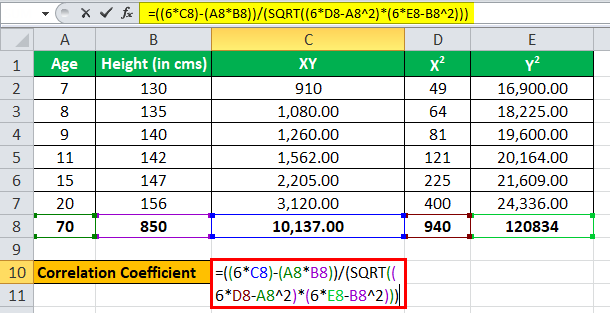
Correlation

Correlation refers to the degree to which two variables move together. In finance, correlation is often used to measure the strength of the relationship between the returns of two different assets, such as stocks or bonds. A correlation coefficient is a statistical measure that quantifies the degree to which the returns of two assets are related.

A correlation coefficient can range from -1 to 1, where -1 represents a perfectly negative correlation (when one asset goes up, the other goes down), 0 represents no correlation (the returns of the two assets are not related), and 1 represents a perfectly positive correlation (when one asset goes up, the other goes up as well).

Correlation is important in portfolio construction because it can help investors to diversify their holdings by selecting assets that have low or negative correlation with each other. This can reduce the overall risk of the portfolio, as losses in one asset may be offset by gains in another. However, it is important to note that correlation is not always stable over time, and can change in response to changes in market conditions or other factors.

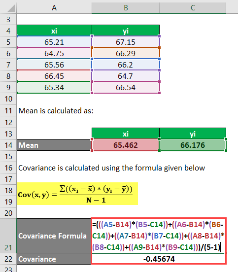
Covariance

Covariance is a statistical measure that quantifies the degree to which two variables move together. In finance, covariance is often used to measure the degree to which the returns of two different assets are related.

Covariance measures the joint variability of two random variables. It is calculated by taking the sum of the product of the difference between each variable's value and its mean, multiplied by the difference between the other variable's value and its mean, and dividing by the total number of observations. A positive covariance indicates that the two variables tend to move together, while a negative covariance indicates that they tend to move in opposite directions.

Covariance is an important input for calculating correlation, which can help investors to diversify their holdings by selecting assets that have low or negative correlation with each other. However, covariance on its own does not provide a standardized measure of the strength of the relationship between two assets, as it is influenced by the scales of the two variables being measured. Correlation, which is derived from covariance, is a more useful measure for assessing the degree to which two assets move together on a standardized scale.

Value at Risk

Value at risk (VaR) is a widely used risk management measure that provides an estimate of the potential loss in the value of an investment or portfolio over a specified time period and at a given level of confidence. VaR is typically expressed as a dollar amount or a percentage of the portfolio's value.

To calculate VaR, statistical methods are used to estimate the potential losses of an investment or portfolio, taking into account the probability of different market scenarios occurring. VaR estimates are based on assumptions about the distribution of returns for the portfolio or investment being analyzed, and can be calculated for different time horizons and levels of confidence.

For example, a 95% VaR estimate for a portfolio of $1 million over a one-month time horizon would indicate that there is a 95% probability that the portfolio will not lose more than a certain dollar amount (the VaR estimate) over the next month.

VaR is used by financial institutions and investors as a risk management tool to assess and control the potential downside risk of their investments. By estimating the potential losses associated with different market scenarios, VaR can help investors and institutions determine how much capital to allocate to specific investments, and how much risk they are willing to take on in their portfolios.

It is important to note that VaR is just one measure of risk, and that it has limitations and assumptions that may not always hold true in practice. As such, VaR should be used in conjunction with other risk measures and risk management techniques to ensure that investors and institutions are adequately managing their risk exposures.

What is value at risk (VaR)? FRM T1-02

Can the standard deviation (volatility) be different from VaR of a portfolio?

Yes. In finance, both standard deviation (SD) and value at risk (VaR) are measures used to assess portfolio risk. SD measures the volatility or dispersion of returns around the portfolio's mean return, while VaR measures the potential loss in value of a portfolio within a specified time frame and at a certain confidence level.

The SD and VaR of a portfolio may differ in the following cases:

Non-normal distribution of returns: If the returns of the portfolio follow a non-normal distribution (i.e., not a bell-shaped curve), then the SD may not accurately reflect the tail risk of the portfolio, which is captured by VaR.

Asymmetric distribution of returns: If the distribution of returns is asymmetric (i.e., skewness or kurtosis is present), then the VaR may capture the downside risk better than SD.

Fat-tailed distribution of returns: If the distribution of returns has fatter tails (i.e., more extreme values than a normal distribution), then the VaR may be a better measure of the downside risk than SD.

Portfolio with nonlinear assets: If the portfolio contains nonlinear assets such as options, then the VaR may be more appropriate as it takes into account the impact of changes in the underlying asset's price on the portfolio.

In summary, the SD and VaR of a portfolio may differ depending on the underlying distribution of returns, skewness or kurtosis, fat tails, and nonlinear assets in the portfolio.

1. Analytical VaR

Analytical VaR (Value at Risk) is a method of calculating the potential loss in value of a portfolio based on statistical analysis. It uses mathematical formulas and statistical models to estimate the risk of a portfolio. Analytical VaR is also known as parametric VaR because it assumes that the distribution of portfolio returns follows a particular probability distribution, typically a normal distribution.

To calculate analytical VaR, the following information is required:

• The expected return of the portfolio
• The standard deviation of the portfolio returns
• The confidence level (typically 95% or 99%)
• The time horizon over which the VaR is to be calculated (e.g., one day or one month)

Using these inputs, analytical VaR can be calculated by taking the expected return of the portfolio and subtracting the product of the standard deviation of the portfolio returns and the corresponding critical value from the normal distribution at the chosen confidence level. This provides an estimate of the maximum potential loss that the portfolio could experience over the chosen time horizon at the chosen confidence level.

Analytical VaR is a widely used method for measuring portfolio risk, particularly for liquid assets with regular market data. However, it does have some limitations, particularly for portfolios with non-normal distributions of returns or those with nonlinear assets.

2. Historical VaR

Historical VaR (Value at Risk) is a method of measuring the potential loss in value of a portfolio based on historical data. It uses the historical returns of a portfolio to estimate the risk of future losses. Unlike analytical VaR, which assumes a probability distribution of returns, historical VaR is a non-parametric approach that does not make any assumptions about the distribution of returns.

To calculate historical VaR, the following steps are typically taken:

Determine the time horizon over which the VaR is to be calculated (e.g., one day or one month)
Select a confidence level (typically 95% or 99%)
Sort the historical returns of the portfolio from worst to best
Determine the historical returns that correspond to the chosen confidence level
The historical VaR is the negative value of the historical return that corresponds to the chosen confidence level
For example, if a portfolio has a 95% historical VaR of $100,000 over a one-day time horizon, this means that there is a 5% chance that the portfolio will lose at least $100,000 in value over the next day based on historical data.

Historical VaR has some advantages over analytical VaR, particularly for portfolios with non-normal distributions of returns or those with nonlinear assets. However, it has limitations as well, particularly when the historical returns do not represent the potential risks of future returns.

3. Monte Carlo Simulation

Monte Carlo simulation is a computational technique used to model and analyze the behavior of complex systems or processes, where there is uncertainty or randomness involved. It is named after the famous casino in Monte Carlo, where games of chance and probability were played.

In Monte Carlo simulation, a model is created that represents the system or process being studied. This model includes the various factors that can affect the outcome, as well as their probabilities of occurrence. The model is then run multiple times using random inputs and the resulting outcomes are recorded. By repeating this process many times, a distribution of possible outcomes can be generated, along with their probabilities of occurrence.

Monte Carlo simulation is often used in finance to model the behavior of financial instruments or portfolios. For example, it can be used to simulate the future returns of a stock or bond portfolio, taking into account the uncertainty and randomness of market movements. It can also be used to estimate the value-at-risk (VaR) of a portfolio, which is a measure of the potential loss that can occur within a given time frame at a certain level of confidence.

Monte Carlo simulation can also be used in other fields, such as engineering, physics, and biology, to model and analyze complex systems and processes. It is a powerful tool for decision-making under uncertainty, as it allows analysts and decision-makers to better understand the range of possible outcomes and their associated probabilities, and to make more informed decisions as a result.

In portfolio construction and bond investing, Monte Carlo simulation can be used to model and analyze the behavior of a portfolio or individual bonds under different scenarios and assumptions. For example, a portfolio manager may want to simulate the future returns of a bond portfolio, taking into account factors such as interest rate changes, credit defaults, and market volatility.

To use Monte Carlo simulation in this context, the portfolio manager would first create a model of the portfolio, including its various components and their characteristics such as duration, credit ratings, and coupon payments. The model would also include assumptions about future market conditions, such as interest rate changes and credit spread movements.

The portfolio manager would then run the Monte Carlo simulation multiple times using random inputs, such as interest rate scenarios and credit spread changes, and record the resulting portfolio returns. By repeating this process many times, a distribution of possible portfolio returns can be generated, along with their probabilities of occurrence.

The portfolio manager can then use this distribution of possible portfolio returns to better understand the range of possible outcomes and their associated probabilities, and to make more informed decisions about portfolio construction and risk management. For example, the portfolio manager may use the results of the simulation to adjust the portfolio's asset allocation, or to evaluate the potential impact of different risk management strategies.

Similarly, Monte Carlo simulation can be used to analyze the behavior of individual bonds under different scenarios and assumptions. For example, a bond investor may want to simulate the future cash flows of a particular bond, taking into account factors such as interest rate changes and credit risk. This can help the investor to better understand the range of possible outcomes and make more informed investment decisions.

In summary, Monte Carlo simulation is a powerful tool for portfolio construction and bond investing, allowing investors and portfolio managers to model and analyze the behavior of their investments under different scenarios and assumptions, and to make more informed decisions as a result.

Shortfall Risk

Shortfall risk is the risk that the actual return on a portfolio will be lower than the expected return or target return. In other words, it is the risk that an investor will experience a loss or a negative deviation from the expected or target return. Shortfall risk is often used in the context of liability-driven investing (LDI), where the investor has a specific future liability to meet, such as pension payments.

Shortfall risk is typically measured as the probability of the actual portfolio return falling below a certain threshold, such as the target return or the return required to meet the future liability. The threshold is often referred to as the "hurdle rate." The greater the probability that the actual return will fall below the hurdle rate, the higher the shortfall risk.

For example, if an investor has a target return of 6% and the probability of the portfolio return falling below 6% is 20%, the investor has a 20% shortfall risk. This means that there is a 20% chance that the investor's portfolio will not meet their target return.

Shortfall risk is an important concept in portfolio management, particularly for investors with future liabilities to meet. By understanding and managing shortfall risk, investors can help ensure that they have sufficient funds to meet their obligations.

In a normal distribution, the expected or target return is represented by the mean of the distribution, while the variability of returns is represented by the standard deviation. Shortfall risk can then be thought of as the probability that the actual return on a portfolio will fall below the target return or "hurdle rate" represented by the mean of the distribution.

For example, let's say an investor has a target return of 8% and the expected return on their portfolio is also 8%, with a standard deviation of 2%. Using a normal distribution, we can calculate the probability of the portfolio return falling below the target return as follows:

The z-score, or the number of standard deviations from the mean, required to meet the target return of 8% is (8% - 8%) / 2% = 0.
The area under the normal curve to the left of the z-score of 0 is 50%. This means that there is a 50% chance that the portfolio return will fall below the target return.
In other words, in a normal distribution, the shortfall risk can be calculated as the probability that the actual return will fall below the target return, based on the mean and standard deviation of the distribution.

Bond Math

Bond Price Calculation: The price of a bond can be calculated using the following formula:

Bond Price = (C / r) x [1 - 1 / (1 + r)^n] + M / (1 + r)^n

Where:

C = coupon payment
r = periodic interest rate
n = number of periods
M = face value or maturity value of the bond

Yield-to-Maturity (YTM) Calculation: The yield-to-maturity is the rate of return an investor would earn if they hold the bond until maturity. It can be calculated using the following formula:

Bond Price = C / (1 + YTM)^1 + C / (1 + YTM)^2 + ... + C / (1 + YTM)^n + M / (1 + YTM)^n

Where:

C = coupon payment
YTM = yield-to-maturity
n = number of periods
M = face value or maturity value of the bond
To solve for YTM, the above equation must be solved for YTM using trial and error or numerical methods.

Current Yield Calculation: The current yield is the annual income earned by the investor as a percentage of the current market price of the bond. It can be calculated using the following formula:

Current Yield = Annual Coupon Payment / Bond Price

Where:

Annual Coupon Payment = coupon payment x number of coupon payments per year
Bond Price = current market price of the bond

Convexity

Convexity is a concept in finance that measures the curvature of the relationship between bond prices and interest rates. It is a measure of how sensitive a bond's price is to changes in interest rates, and how that sensitivity changes as interest rates move up or down.

In general, when interest rates rise, the price of a bond falls, and when interest rates fall, the price of a bond rises. However, the relationship between bond prices and interest rates is not always linear - in other words, the price change of a bond is not always proportional to the change in interest rates.

Convexity measures the extent to which this relationship is curved or "convex". Specifically, it measures the second derivative of the bond price with respect to changes in interest rates. A bond with higher convexity will have a more curved price-yield relationship, meaning that its price will be less sensitive to changes in interest rates when rates are low, but more sensitive when rates are high.

Convexity is an important factor to consider when investing in bonds, because it affects the risk and return characteristics of a bond or a bond portfolio. Bonds with higher convexity tend to have higher prices and lower yields than bonds with lower convexity, all else equal. However, they also tend to have higher price volatility, meaning that their prices can fluctuate more widely in response to changes in interest rates.

In summary, convexity is a measure of the curvature of the relationship between bond prices and interest rates. It is an important factor to consider when investing in bonds, as it affects the risk and return characteristics of a bond or a bond portfolio.

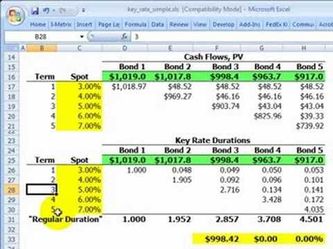
Key Rate Duration (KRD)

The concept of key rate duration is closely related to convexity in bond investing. Key rate duration is a measure of the sensitivity of a bond's price to changes in specific "key" interest rates, rather than changes in interest rates across the entire yield curve.

Key rate duration is calculated by decomposing a bond's total duration into its component parts, each of which measures the bond's sensitivity to changes in a particular key rate. The key rates used for this calculation are typically the rates on benchmark government bonds at specific maturities along the yield curve.

The concept of key rate duration comes into play in relation to convexity because it helps investors to better understand how a bond's price will change under different interest rate scenarios, particularly if interest rates change unevenly across the yield curve. For example, if short-term interest rates are expected to rise while long-term interest rates are expected to remain stable, a bond's key rate duration would help to reveal the bond's sensitivity to the rising short-term rates, and therefore provide a more accurate picture of its overall price sensitivity.

Convexity also comes into play in relation to key rate duration, because it affects the sensitivity of a bond's price to changes in the key rates. Specifically, as interest rates change, the relationship between a bond's price and its key rate durations can become more or less convex. Bonds with higher convexity will experience more pronounced price changes due to changes in key rates, while bonds with lower convexity will experience smaller price changes.

Therefore, investors who are interested in managing interest rate risk in their bond portfolios need to consider both key rate duration and convexity to fully understand the impact of changes in interest rates on bond prices. By doing so, they can make more informed investment decisions and manage their risk exposure more effectively.

The formula for key rate duration is as follows:

Key Rate Duration = -[(P-) - (P+)] / 2 * (Δy)

Where:

P- is the bond price when the key rate is decreased by a small amount (Δy)
P+ is the bond price when the key rate is increased by the same amount (Δy)
Δy is the change in the specific key interest rate used to calculate the key rate duration
The key rate duration formula is used to calculate the sensitivity of a bond's price to changes in specific key interest rates along the yield curve. The formula helps investors to better understand how a bond's price will change under different interest rate scenarios, particularly if interest rates change unevenly across the yield curve.

Calculation

• Key Rate Shift (9 min)

• Key Rate Shift Technique (30 min)
• Key Rate Duration using R code (blog)

Bond Risk Measures

1. Interest rate risk: This is the risk that changes in interest rates will affect the value of the bond. Generally, when interest rates rise, bond prices fall, and when interest rates fall, bond prices rise.

To measure interest rate risk,

• Duration: Duration is a measure of the sensitivity of a bond's price to changes in interest rates. The higher the duration, the more sensitive the bond's price is to changes in interest rates.
• Convexity: Convexity is a measure of how the duration of a bond changes as interest rates change. It provides a more accurate estimate of the bond's price sensitivity to interest rate changes than duration alone.
• Yield curve risk: This is the risk that changes in the shape of the yield curve, which represents the relationship between yields and maturities of bonds, will affect the value of a bond or portfolio of bonds.
• Basis risk: Basis risk arises when the value of a bond or portfolio of bonds is affected by changes in the relationship between different interest rates, such as the spread between short-term and long-term interest rates.
• Optionality risk: Optionality risk arises from embedded options in bonds, such as call options, which allow the issuer to redeem the bond early. This can cause uncertainty about the timing of cash flows and affect the value of the bond.
• Credit spread risk: Credit spread risk is the risk that the difference between the yield of a bond and a benchmark interest rate, such as the yield on government bonds, will widen, affecting the value of the bond.

2. Credit risk: This is the risk that the bond issuer will default on its debt obligations, or become unable to pay the interest or principal payments as scheduled. Bonds issued by companies with lower credit ratings are generally considered to have higher credit risk.

To measure credit risk,

• Credit ratings: Credit ratings assigned by credit rating agencies such as Standard & Poor's, Moody's, and Fitch are widely used as a measure of credit risk. Higher-rated bonds are generally considered to have lower credit risk.
• Default probability: Default probability is a statistical measure of the likelihood that a bond issuer will default on its debt obligations. It is based on factors such as the issuer's financial health, operating environment, and market conditions.
• Credit spread: The credit spread is the difference between the yield of a bond and a benchmark interest rate, such as the yield on government bonds. A wider credit spread indicates a higher perceived credit risk.
• Recovery rate: The recovery rate is the percentage of the bond's face value that the investor can expect to recover in the event of a default. A lower recovery rate indicates higher credit risk.
• Covenants: Bond covenants are contractual terms that specify certain obligations and restrictions on the issuer. Stronger covenants, such as those that require the issuer to maintain certain financial ratios or limit the amount of debt it can issue, can reduce credit risk.

3. Inflation risk: This is the risk that inflation will erode the purchasing power of the bond's future cash flows, such as interest payments and principal repayment.

To measure inflation risk,

• Real interest rates: Real interest rates are nominal interest rates adjusted for inflation. They represent the true cost of borrowing or the true return on investment. Inflation risk is higher when real interest rates are low or negative.
• Inflation expectations: Inflation expectations are the market's forecast of future inflation. Higher inflation expectations indicate higher inflation risk, and vice versa.
• Duration: Duration is a measure of the sensitivity of a bond's price to changes in interest rates. Duration can also be used as a measure of inflation risk, as inflation can lead to changes in interest rates.
• Index-linked bonds: Index-linked bonds, also known as inflation-linked bonds or real return bonds, are bonds whose payments are adjusted for inflation. The yield on index-linked bonds can be used as a measure of inflation expectations.
• Consumer Price Index (CPI): The CPI is a measure of the average change over time in the prices paid by consumers for a basket of goods and services. Changes in the CPI can be used as a measure of actual inflation and can be compared to inflation expectations.

4. Call risk: This is the risk that the issuer will redeem the bond before its maturity date, usually in a declining interest rate environment, leaving investors with reinvestment risk.

To measure call risk,

• Yield-to-call (YTC): YTC is the yield that an investor would receive if the bond were called at the earliest possible date. A lower YTC indicates higher call risk, as the bond is more likely to be called and the investor may miss out on future interest payments.
• Yield-to-worst (YTW): YTW is the yield that an investor would receive if the bond were called at the worst possible time, taking into account all possible call dates and prices. YTW provides a more conservative estimate of the bond's yield and can be used as a measure of call risk.
• Call option-adjusted spread (OAS): OAS is the difference between the yield of a bond and the yield of a similar, risk-free bond, adjusted for the value of any embedded call options. A wider OAS indicates higher call risk, as the issuer may be more likely to exercise its call option and redeem the bond.
• Weighted average call date (WACD): WACD is the average call date of all possible call dates, weighted by the amount of principal that would be redeemed if the bond were called on each date. A shorter WACD indicates higher call risk, as the issuer has more opportunities to call the bond.

5. Liquidity risk: This is the risk that the bond cannot be sold easily in the market at a fair price, or the market is too small or illiquid to accommodate large transactions.

To measure liquidity risk,

• Bid-ask spread: The bid-ask spread is the difference between the highest price a buyer is willing to pay (bid) and the lowest price a seller is willing to accept (ask). A wider bid-ask spread indicates lower liquidity and higher liquidity risk.
• Trading volume: Trading volume refers to the number of shares or bonds traded in a given period. Higher trading volume indicates higher liquidity and lower liquidity risk.
• Market depth: Market depth refers to the availability of buyers and sellers at different prices. Deeper markets have more buyers and sellers, providing greater liquidity and lower liquidity risk.
• Time to execute: Time to execute is the time it takes to buy or sell a security. Longer time to execute indicates lower liquidity and higher liquidity risk.
• Size of the position: The size of the position refers to the number of shares or bonds held by an investor. Larger positions can be more difficult to sell quickly without affecting the price, indicating higher liquidity risk.

6. Currency risk: This is the risk that exchange rate fluctuations will affect the value of a bond denominated in a foreign currency, especially if the investor's home currency strengthens against the foreign currency.

To measure currency risk,

• Currency volatility: Currency volatility refers to the extent to which the value of a currency fluctuates over time. Higher volatility indicates higher currency risk, as the value of the investment may be more unpredictable.
• Correlation with the domestic currency: The correlation between the investment's currency and the investor's domestic currency can affect the risk of the investment. If the currencies are highly correlated, fluctuations in the investment's currency may have less impact on the investment's value.
• Hedging options: Hedging refers to using financial instruments to mitigate currency risk. The availability of hedging options can affect the level of currency risk associated with an investment.
• Country risk: Country risk refers to the risk of political or economic instability in the country where the investment is located. Higher country risk can increase currency risk, as currency values may be more affected by changes in the country's political or economic environment.
• Interest rate differentials: Interest rate differentials between countries can affect currency values. Higher interest rates in one country can lead to increased demand for its currency, which can cause the currency to appreciate relative to other currencies.

Performance measures

• Return: This measures the percentage change in the value of the portfolio over a given period of time. It is the most commonly used performance measure and provides a simple way to compare the performance of different portfolios.
• Risk-adjusted return: This measures the return of the portfolio relative to the level of risk taken on to achieve that return. Common risk-adjusted return measures include the Sharpe ratio, the Treynor ratio, and Jensen's alpha.

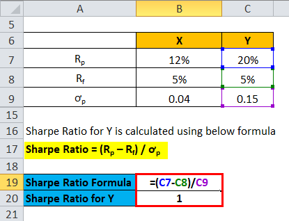
1. Sharpe ratio: This is a measure of the excess return per unit of risk taken on by the portfolio, relative to a risk-free asset. It is calculated as the portfolio's excess return over the risk-free rate, divided by the portfolio's standard deviation of returns. A higher Sharpe ratio indicates better risk-adjusted returns.

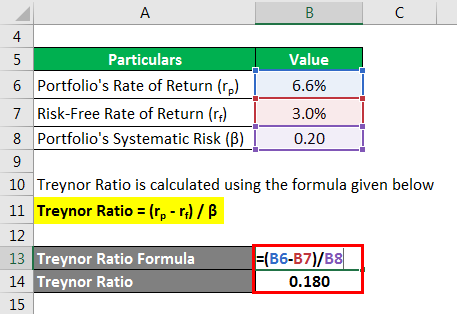
2. Treynor ratio: This is similar to the Sharpe ratio, but instead of using the portfolio's standard deviation of returns, it uses the portfolio's beta (systematic risk). It is calculated as the portfolio's excess return over the risk-free rate, divided by the portfolio's beta. A higher Treynor ratio indicates better risk-adjusted returns.

3. Jensen's alpha: This measures the excess return of the portfolio relative to its expected return, based on its level of risk (beta). It is calculated as the portfolio's actual return minus the expected return (based on the capital asset pricing model or CAPM), adjusted for the portfolio's beta and the risk-free rate. A positive Jensen's alpha indicates that the portfolio has outperformed its expected return based on its level of risk.

Explainer: Sharpe ratio, Treynor ratio, M2 , and Jensen’s alpha

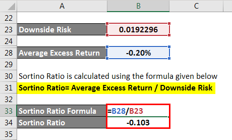
4. Sortino ratio: It is similar to the Sharpe ratio, but it uses downside deviation rather than standard deviation to calculate risk.

The downside deviation is a measure of the volatility of returns below a certain threshold or minimum acceptable return, typically the risk-free rate or the minimum required return for an investment. The Sortino ratio is calculated by taking the excess return of the investment or portfolio over the minimum acceptable return, and dividing it by the downside deviation.

The Sortino ratio is useful for evaluating investments or portfolios that have a higher frequency of downside volatility or losses, as it penalizes the investment for downside volatility while ignoring upside volatility. This makes it a more appropriate measure for evaluating investments with a skewed distribution of returns, such as hedge funds or private equity funds. A higher Sortino ratio indicates a better risk-adjusted performance.

• Volatility: This measures the degree of variation of the portfolio's returns over a given period of time. Volatility is often measured using standard deviation.
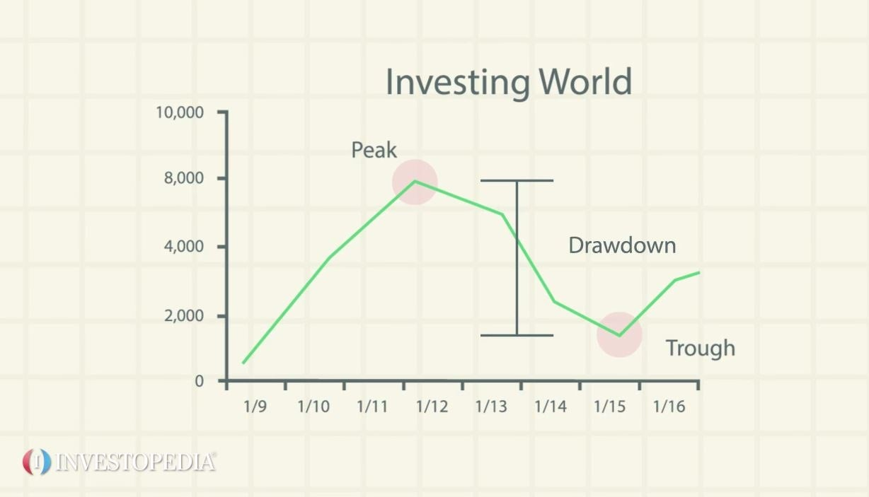
• Drawdown: This measures the peak-to-trough decline in the value of the portfolio over a given period of time. It provides an indication of the largest loss that an investor would have experienced if they had invested in the portfolio at its peak value.

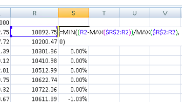
Calculating max drawdown and drawdown on spreadsheet

• Tracking error: This measures the degree of deviation of the portfolio's returns from its benchmark. A lower tracking error indicates that the portfolio is closely following its benchmark.

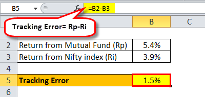
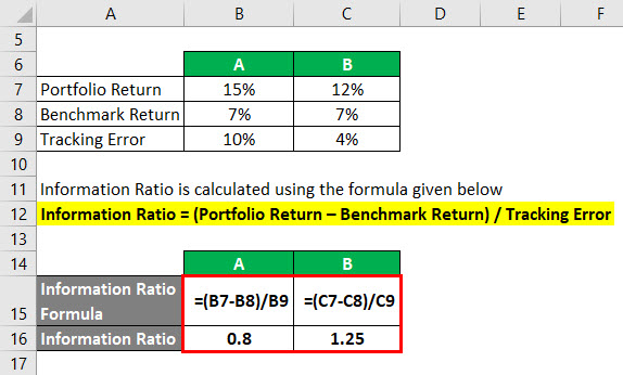
• Information ratio: This measures the portfolio's risk-adjusted return relative to its benchmark, taking into account the tracking error.

Other Suggested Resources

Risk Foundations (FRM T1-01) playlist